7. Co-location
One of the key features of the Community Intercomparison Suite (CIS) is the ability to co-locate one or more arbitrary data sets onto a common set of coordinates. This page briefly describes how to perform co-location in a number of scenarios.
To perform co-location, run a command of the format:
$ cis col <datagroup> <samplegroup> -o <outputfile>
where:
<datagroup>is a CIS datagroup specifying the variables and files to read and is of the format
<variable>...:<filename>[:product=<productname>]where:<variable>is a mandatory variable or list of variables to use.<filenames>is a mandatory file or list of files to read from.<productname>is an optional CIS data product to use (see Data Products):
See Datagroups for a more detailed explanation of datagroups.
<samplegroup>is of the format
<filename>[:<options>]The available options are described in more detail below. They are entered in a comma separated list, such asvariable=Temperature,colocator=bin,kernel=mean. Not all combinations of colocator and data are available; see Available Colocators.<filename>is a single filename with the points to colocate onto.variableis an optional argument used to specify which variable’s coordinates to use for colocation. If a variable is specified, a missing value will be set in the output file at every point for which the sample variable has a missing value. If a variable is not specified, non-missing values will be set at all sample points unless colocation at a point does not result in a valid value.colocatoris an optional argument that specifies the colocation method. Parameters for the colocator, if any, are placed in square brackets after the colocator name, for example,colocator=box[fill_value=-999,h_sep=1km]. If not specified, a Default Colocator is identified for your data / sample combination. The colocators available are:binFor use only with ungridded data and gridded sample points. Data points are placed in bins corresponding to the cell bounds surrounding each grid point. The bounds are taken from the gridded data if they are defined, otherwise the mid-points between grid points are used. The binned points should then be processed by one of the kernels to give a numeric value for each bin.boxFor use with gridded and ungridded sample points and data. A search region is defined by the parameters and points within the defined separation of each sample point are associated with the point. The points should then be processed by one of the kernels to give a numeric value for each bin. The parameters defining the search box are:h_sep- the horizontal separation. The units can be specified as km or m (for exampleh_sep=1.5km); if none are specified then the default is km.a_sep- the altitude separation. The units can be specified as km or m, as for h_sep; if none are specified then the default is m.p_sep- the pressure separation. This is not an absolute separation as for h_sep and a_sep, but a relative one, so is specified as a ratio. For example a constraint of p_sep = 2, for a point at 10 hPa, would cover the range 5 hPa < points < 20 hPa. Note that p_sep >= 1.t_sep- the time separation. This can be specified in years, months, days, hours, minutes or seconds usingPnYnMnDTnHnMnS(the T separator can be replaced with a colon or a space, but if using a space quotes are required). For example to specify a time separation of one and a half months and thirty minutes you could uset_sep=P1M15DT30M. It is worth noting that the units for time comparison are fractional days, so that years are converted to the number of days in a Gregorian year, and months are 1/12th of a Gregorian year.
If
h_sepis specified, a k-d tree index based on longitudes and latitudes of data points is used to speed up the search for points. It h_sep is not specified, an exhaustive search is performed for points satisfying the other separation constraints.linFor use with gridded source data only. A value is calculated by linear interpolation for each sample point.nnFor use with gridded source data only. The data point closest to each sample point is found, and the data value is set at the sample point.dummyFor use with ungridded data only. Returns the source data as the colocated data irrespective of the sample points. This might be useful if variables from the original sample file are wanted in the output file but are already on the correct sample points.
Colocators have the following general optional parameters, which can be used in addition to any specific ones listed above:
fill_value- The numerical value to apply to the colocated point if there are no points which satisfy the constraint.var_name- Specifies the name of the variable in the resulting NetCDF file.var_long_name- Specifies the variable’s long name.var_units- Specifies the variable’s units.
kernelis used to specify the kernel to use for colocation methods that create an intermediate set of points for further processing, that is box and bin. The default kernel for box and bin is moments. The built-in kernel methods currently available are:moments- Default. This is an averaging kernel that returns the mean, standard deviation and the number of points remaining after the specified constraint has been applied. This can be used for gridded or ungridded sample points where the colocator is one of ‘bin’ or ‘box’. The names of the variables in the output file are the name of the input variable with a suffix to identify which quantity they represent:- Mean - no suffix - the mean value of all data points which were mapped to that sample grid point (data points with missing values are excluded)
- Standard Deviation - suffix:
_std_dev- The corrected sample standard deviation (i.e. 1 degree of freedom) of all the data points mapped to that sample grid point (data points with missing values are excluded) - Number of points - suffix:
_num_points- The number of data points mapped to that sample grid point (data points with missing values are excluded)
mean- an averaging kernel that returns the mean values of any points found by the colocation methodnn_t(ornn_time) - nearest neighbour in time algorithmnn_h(ornn_horizontal) - nearest neighbour in horizontal distancenn_a(ornn_altitude) - nearest neighbour in altitudenn_p(ornn_pressure) - nearest neighbour in pressure (as in a vertical coordinate). Note that similarly to thep_sepconstraint that this works on the ratio of pressure, so the nearest neighbour to a point with a value of 10 hPa, out of a choice of 5 hPa and 19 hPa, would be 19 hPa, as 19/10 < 10/5.
productis an optional argument used to specify the type of files being read. If omitted, the program will attempt to determine which product to use based on the filename, as listed at Reading.
<outputfile>- is an optional argument specifying the file to output to. This will be automatically given a
.ncextension if not present and if the output is ungridded, will be prepended withcis-to identify it as a CIS output file. This must not be the same file path as any of the input files. If not provided, the default output filename is out.nc
A full example would be:
$ cis col rain:"my_data_??.*" my_sample_file:colocator=box[h_sep=50km,t_sep=6000S],kernel=nn_t -o my_col
Warning
When colocating two data sets with different spatio-temporal domains, the sampling points should be within the spatio-temporal domain of the source data. Otherwise, depending on the co-location options selected, strange artefacts can occur, particularly with linear interpolation. Spatio-temporal domains can be reducded in CIS with Aggregation or Subsetting.
7.1. Available Colocators and Kernels
| Colocation type | |||
|---|---|---|---|
| ( data -> sample) | Available Colocators | Default Colocator | Default Kernel |
| Gridded -> gridded | lin, nn, box |
lin |
None |
| Ungridded -> gridded | bin, box |
bin |
moments |
| Gridded -> ungridded | nn, lin |
nn |
None |
| Ungridded -> ungridded | box |
box |
moments |
7.2. Colocation output files
All ungridded co-location output files are prefixed with cis- and both ungridded and gridded data files are suffixed with .nc (so there is no need to specify the extension in the output parameter). This is to ensure the cis data product is always used to read co-located ungridded data.
It is worth noting that in the process of colocation all of the data and sample points are represented as 1-d lists, so any structural information about the input files is lost. This is done to ensure consistency in the colocation output. This means, however, that input files which may have been plotable as, for example, a heatmap may not be after co-location. In this situation plotting the data as a scatter plot will yield the required results.
Each co-located output variable has a history attributed created (or appended to) which contains all of the parameters and file names which went into creating it. An example might be:
double mass_fraction_of_cloud_liquid_water_in_air(pixel_number) ;
    ...
    mass_fraction_of_cloud_liquid_water_in_air:history = "Colocated onto sampling from:   [\'/test/test_files/RF04.20090114.192600_035100.PNI.nc\'] using CIS version V0R4M4\n",
        "variable: mass_fraction_of_cloud_liquid_water_in_air\n",
        "with files: [\'/test/test_files/xenida.pah9440.nc\']\n",
        "using colocator: DifferenceColocator\n",
        "colocator parameters: {}\n",
        "constraint method: None\n",
        "constraint parameters: None\n",
        "kernel: None\n",
        "kernel parameters: None" ;
    mass_fraction_of_cloud_liquid_water_in_air:shape = 30301 ;
double difference(pixel_number) ;
    ...
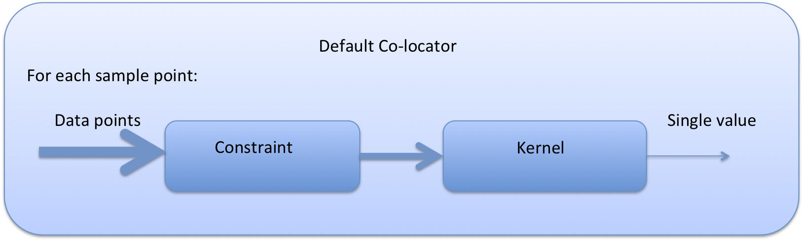
7.3. Basic colocation design
The diagram below demonstrates the basic design of the co-location system, and the roles of each of the components. In the simple case of the default co-locator (which returns only one value) the Colocator loops over each of the sample points, calls the relevant constraint to reduce the number of data points, and then the kernel which returns a single value which the co-locator stores.
It is useful to understand that when a sample variable is specified that contains masked values (those with a fill_value) this is not taken into account when creating the list of sample points. E.g. the full list of coordinates is used from the file, regardless of the values of the sample variable.
On the contrary when a data variable is read in (which is to be co-located onto the sample) any masked values are ignored. That is, any value in the data variable which is equal to the fill_value is not considered for colocation, as it is treated as an empty value.
On their own each of these statements seem sensible, but together may lead to unexpected results if, for example, a variable from a file is co-located onto itself using the DefaultColocator. In this situation, the sampling from the file is used to determine the sample points regardless of fill_value, and the variable is co-located on to this (ignoring any fill_values). This results in an output file where the masked (or missing) values are ‘filled-in’ by the co-locator using whichever kernel was specified - see Figure 2a below. Using the DummyColocator simply returns the original masked values as no filling in is done (see 2b), and similarly for the difference co-locator when co-located onto itself the difference variable retains the mask as a non-value minus any other number is still a non-value (see 2c).
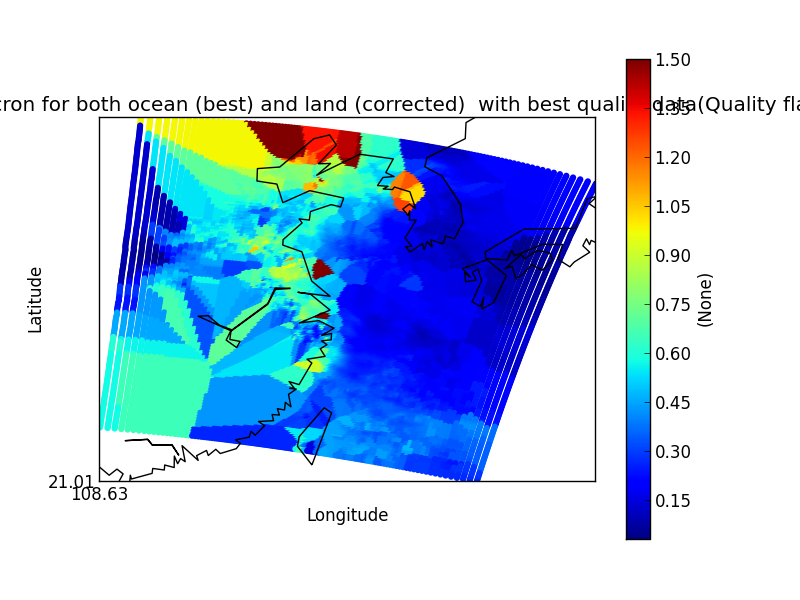
Figure 2a
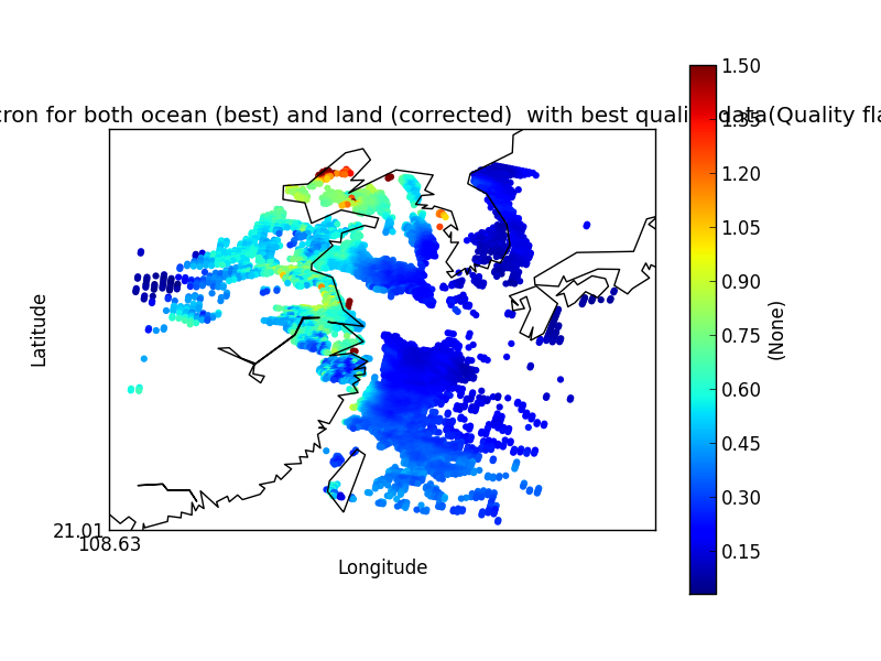
Figure 2b
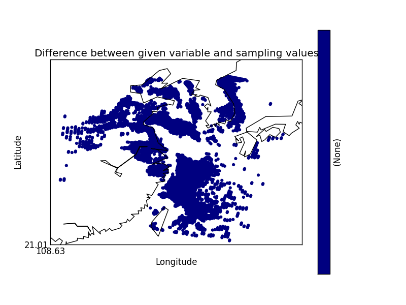
Figure 2c
7.4. Writing your own plugins
The colocation framework was designed to make it easy to write your own plugins. Plugins can be written to create new kernels, new constraint methods and even whole colocation methods. See Colocation Design for more details